


By Mark Caslin, CEO, Alder Capital
Uses of volatility forecasting in financial markets
Volatility is generally accepted as the best measure of market risk and volatility forecasting is used in many different applications across the industry. These include risk management, VAR, portfolio construction and optimisation, active fund management, risk-parity investing, and derivatives trading. Implementing a market risk forecast is also becoming an ever more important feature of the regulatory environment, as seen in the risk-rating of investment products through ESMA, PRIIPS or IORP II. Accurately modelling volatility is of significant value.
Standard approaches to volatility forecasting
A good model of volatility should capture two key features observed in the real world.
- Conditionality feature - successive days tend to be similarly higher than average (or lower) – volatility clusters.
- Autoregressive feature - volatility exhibits long memory where levels tend to mean revert to longer run values.
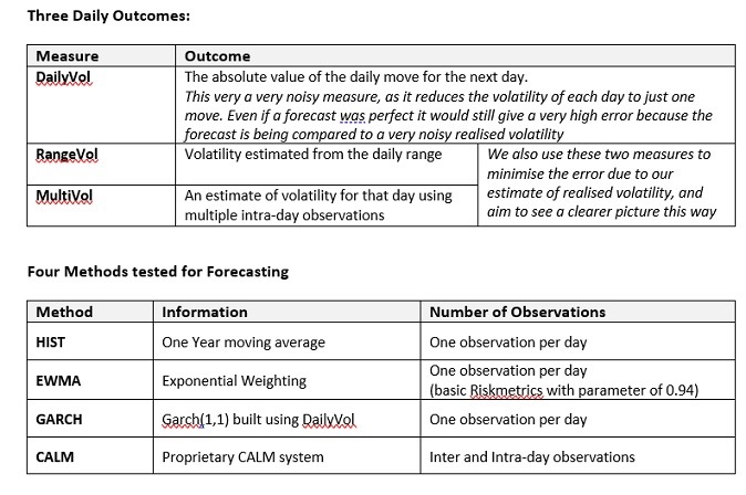
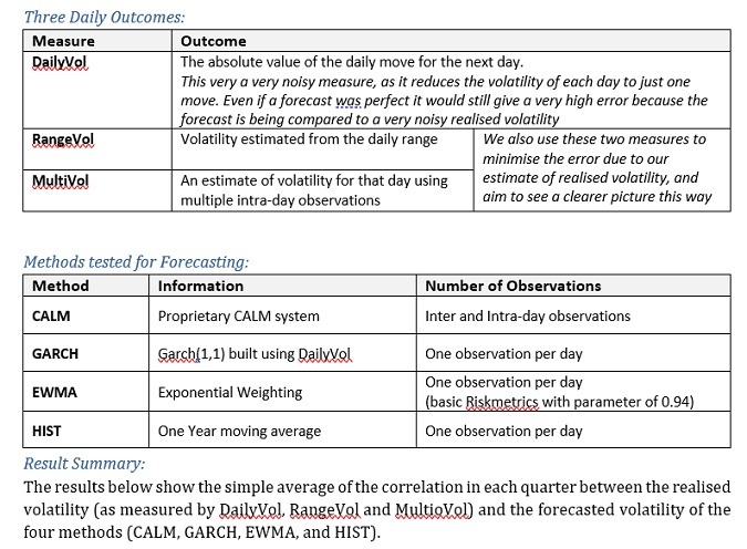
Volatility modelling is a complex subject and a multitude of solutions have been proposed. In practice, the industry has condensed onto three main techniques:
- Historical Average (HIST)
Typically uses the previous year’s volatility as a forecast for the next period. When volatility moves to a new level this method can be too slow to react. For example, if volatility were to double it would take this method 5 months to move halfway to the new level.
- Exponentially Weighted Moving Average (EWMA)
Takes an average of previous days volatilities, with exponentially declining weights - so older data gets rapidly less important. A decay rate of 0.94 is commonly used (Original RiskMetrics) and this approach can indeed capture volatility clustering. It suffers, however, as the better it is at capturing the Conditionality feature the worst it is at capturing the Autoregressive feature.
- GARCH
Captures both clustering and mean reversion because it has parameters for both. It has a decay feature similar to EWMA but with a long-term average parameter thus 'dragging volatility back' to a longer run value. In-sample, this approach can be an excellent fit, but its ability to forecast is often little better than the much simpler EWMA method. The key problem is that GARCH has three parameters so it can often fit very well but it is often an overfit and it may not be a good forecast. In addition, applied to a multi asset situation it can imply unreliable correlations when each asset is parameterised separately.
Variations
There are many variations of the above models which attempt to overcome the many drawbacks but while their increased complexity fits the in-sample data better it doesn't always result in improved forecast accuracy out of sample. One of the reasons is that the quality of the output can’t be better than the quality of the input and the input is typically the daily move which has high variability. It is very hard for any method to accurately converge to a new volatility level when the input observations are so variable.
The CALM model
To Forecast volatility, Alder Capital uses a proprietary multi-point method, per day, as inputs to its CALM system. It builds on statistical techniques to deliver a one-day ahead forecast. The technique captures long memory effects and harnesses the power of both inter and intra-day data. The system has been developed over many years as a key component of the Alder Capital investment process. It has evolved and been continuously refined through direct implementation, resulting in superior forecasting accuracy.
Assessing Accuracy of Volatility Forecasting Models
In order to measure the accuracy of the CALM system in forecasting volatility, we need to compare the forecast with realised volatility, on a daily basis. This poses a question as to what is meant by “realised volatility” for one day. So, for this analysis, we use three common measures to assess performance:
Three Daily Outcomes:
Investigation Setup
- It’s important to note, that each forecast only uses data available prior to that day.
- Time snapshot 3:00pm.
- We examine the “surprise” risk in each of the four volatility forecasting methods. A good forecasting method would have fewer “surprises” i.e. fewer outcomes that were unlikely considering our forecast.
- We consider each of the three daily outcomes against each of the four forecasting methods.
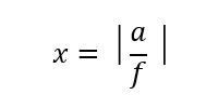
- The question is, how does the actual outcome, compare with the forecast. Let ‘a’ be the absolute value of the actual daily outcome with an associated forecast ‘f’, then our observed statistic would be ‘x’ where:
- Confidence interval @ 95%
- Outliers Measurements
We choose three critical points (x1, x2 & x3), one for each of the three daily outcome methods (DailyVol, RangeVol & MultiVol), that corresponds to where the CALM method has 2.5% of its daily realised outcomes above that point and 2.5% of its daily realised outcomes below that point. We measure how often the other methods exceed that same critical value. This tells us how often the methods give an outcome outside a 95% confidence interval.
Comparing how many outliers each of the forecasting methods have will help determine which approach is better at forecasting volatility.
S&P 500 Analysis
Our out of sample forecasts start on January 1st, 2007 and go through to December 31st, 2019. It’s important to note, that each forecast only uses data available prior to that day.
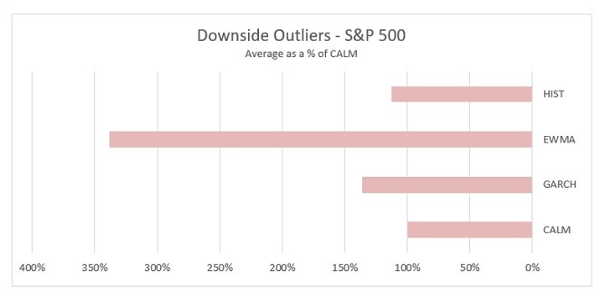
The tables below show the percentage of outcomes above/below the critical values for the three daily outcomes and the four volatility forecasting methods. In the final column it shows the average number of outliers as a % of the CALM method’s number of outliers, across the three daily outcomes.
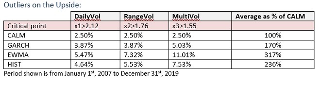
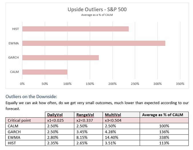
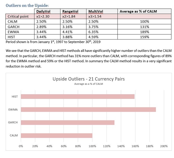
We see in the chart below that the GARCH, EWMA and HIST methods all have significantly higher number of outliers than the CALM method. In particular, the GARCH method has 70% more outliers than CALM, with corresponding figures of 217% for the EWMA method and 136% or the HIST method. In summary the CALM method results in a very significant reduction in outlier risk.
Period shown is from January 1st, 2007 to December 31st, 2019
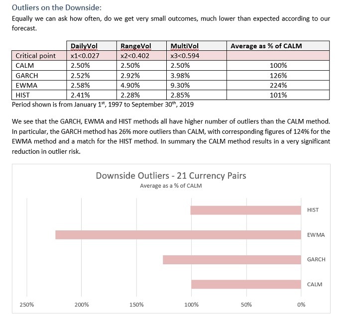
We see in the chart below that the GARCH, EWMA and HIST methods all have higher number of outliers than the CALM method. In particular, the GARCH method has 36% more outliers than CALM, with corresponding figures of 238% for the EWMA method and 13% or the HIST method. In summary the CALM method results in a very significant reduction in outlier risk.
S&P 500 Analysis Notes
- The HIST method performs well at reducing surprises on the low side, but its weakness is surprises on the upside.
- The EWMA is poor at both, as exponential weighting can’t capture an autoregressive and a conditional feature at the same time.
- GARCH has an average of about 53% more outliers across the downside and the upside.
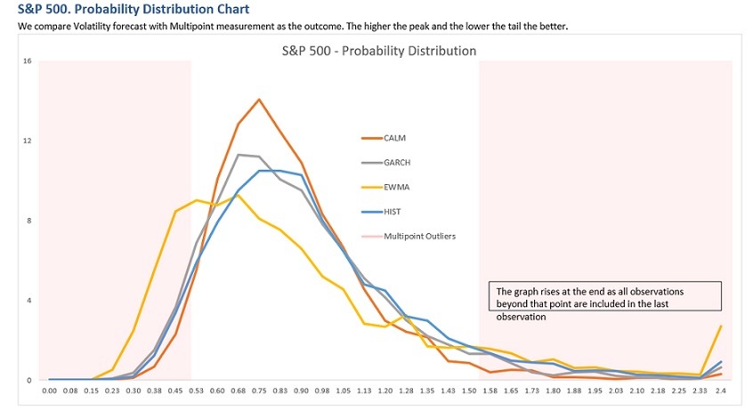
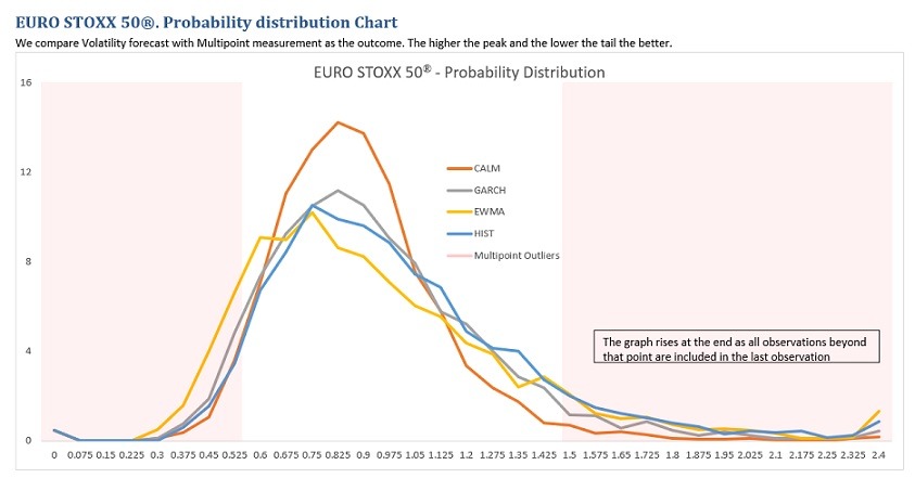
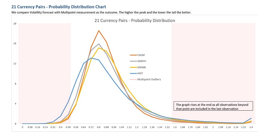
We compare Volatility forecast with Multipoint measurement as the outcome. The higher the peak and the lower the tail the better.
EURO STOXX 50® Analysis
Our out of sample forecasts start on January 1st, 2007 and go through to December 31st, 2019. It’s important to note, that each forecast only uses data available prior to that day.
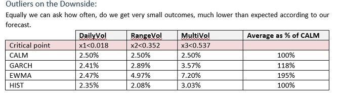
The tables below show the percentage of outcomes above/below the critical values for the three daily outcomes and the four volatility forecasting methods. In the final column it shows the average number of outliers as a % of the CALM method’s number of outliers, across the three daily outcomes.
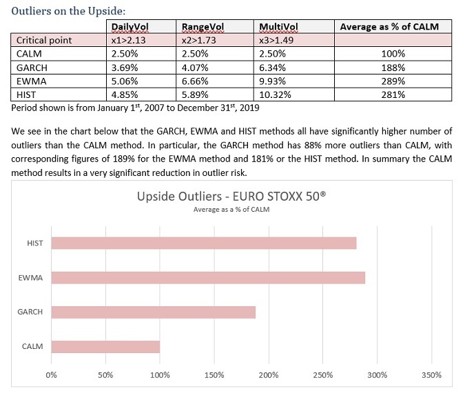
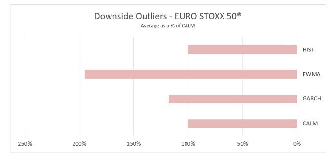
Period shown is from January 1st, 2007 to December 31st, 2019
We see in the chart below that the GARCH, EWMA and HIST methods all have higher number of outliers than the CALM method. In particular, the GARCH method has 18% more outliers than CALM, with corresponding figures of 95% for the EWMA method and a match for the HIST method. In summary the CALM method results in a very significant reduction in outlier risk.
- The HIST method performs well at reducing surprises on the low side, but its weakness is surprises on the upside.
- The EWMA is poor at both, as exponential weighting can’t capture an autoregressive and a conditional feature at the same time.
- GARCH has an average of about 53% more outliers across the downside and the upside.
Currency Analysis
Our out-of-sample forecasts start on January 1st, 1997 to September 30th, 2019. It’s important to note, that each forecast only uses data available prior to that day.
We use the following currencies: EUR, USD, JPY, GBP, CAD, AUD and SEK to create 21 currency pairs (all the crosses) to include in our analysis. Calm uses the same parameters for every currency, so we have no positive definite problems. GARCH is built per currency pair so it has an advantage in each pair however, it has the downside that the correlations between currency pairs can’t be relied up, it may imply that you can create portfolios with negative volatility, volatility black holes if you like.
The tables below show the percentage of outcomes above/below the critical values for the three daily outcomes and the four volatility forecasting methods. In the final column it shows the average number of outliers as a % of the CALM method’s number of outliers, across the three daily outcomes.
Notes on Currency Analysis
- The HIST method performs well at reducing surprises on the low side, but its weakness is surprises on the upside.
- The EWMA is poor at both, as exponential weighting can’t capture an autoregressive and a conditional feature at the same time.
- GARCH has about 28% more outliers on both the downside and the upside.
Conclusion
Our analysis covers the S&P 500 index and the EURO STOXX 50® index over a 13-year period and 21 currency pairs, over a 23-year period, all including the global financial crisis.
Against each of the three daily outcome measures we see that the current industry standard methods have a significantly higher number of outliers, about 50% in the two equity indices and about 30% across the 21 currency pairs.
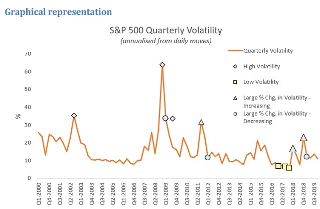
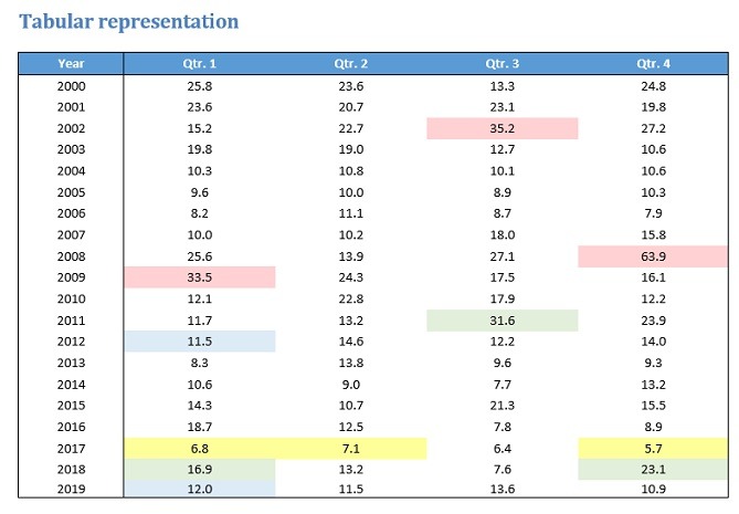
Comparing Volatility Systems Across Difficult Quarters
Analysing the last 20 years, between Q1 2000 to Q4 2019, we looked at the performance of each of the volatility forecasting models during difficult quarters.
We divided these difficult quarters into 4 categories and chose the top 3 quarters in each category as sample outputs:
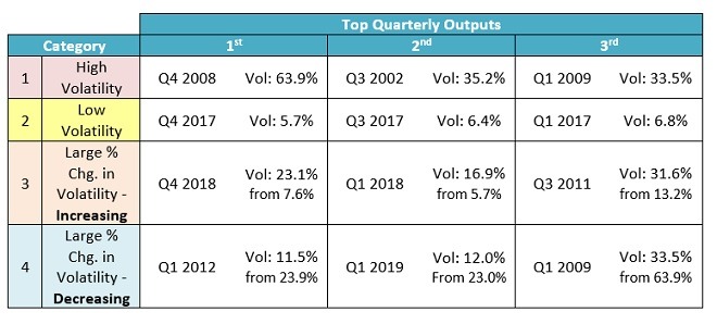
For this purpose, we measure volatility from daily changes. There is one quarter, Q1 2019, which shows up twice, however we only include it once in the analysis, so we use 11 quarters as shown in the graph and table below.
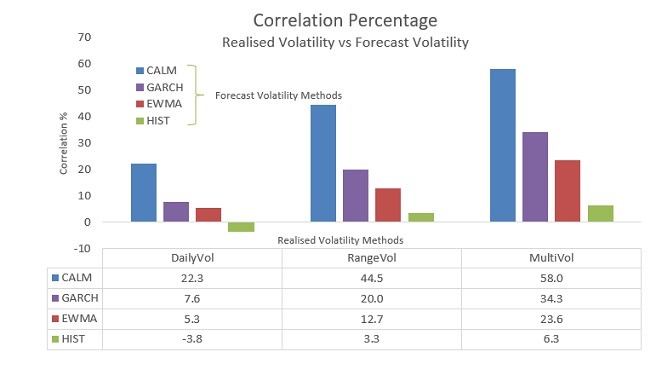
Correlation Analysis
For each of the quarters chosen we calculate the correlation of the actual realised volatility per day with the forecast of volatility for that day.
Realised volatility is measured in three different ways.
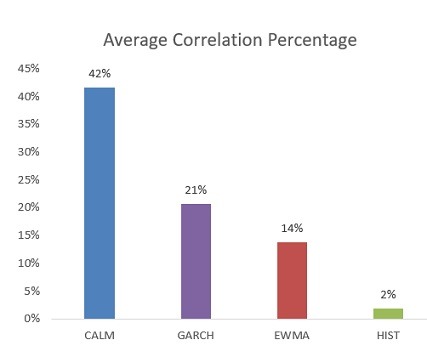
Summary
We see that the CALM method is better irrespective of how you measure realised volatility. In particular, we can see that on average, across the difficult quarters and across the different realised volatility measures, CALM has 100% better correlation between the forecasted volatility and the realised volatility than the next best method, GARCH.
Source: Alder Capital DAC unless otherwise stated. The data and calculations are not necessarily audited or independently verified.
Caution: The information in this document is not to be construed as an offer to buy or sell or a solicitation of an offer to buy or sell any financial instrument or to participate in any trading strategy in any jurisdiction in which such an offer or solicitation would violate applicable laws or regulations. Alder Capital is not soliciting any action based on this document.
The information in this document does not constitute investment, accounting, credit, taxation, regulatory or legal advice. It does not take into account the investment objectives, financial position or particular needs of any particular investor. If you intend entering into an investment management agreement with Alder Capital you should consult suitably qualified and independent investment, taxation, accounting, legal and regulatory advisors to discuss your specific situation and investment objectives before proceeding. Trading strategies and financial instruments discussed in this document are not suitable for all investors.
Opinions, estimates and projections in this document constitute Alder Capital’s judgement as of the date of this document and are subject to change without notice.
Contact Mark Caslin at mark.caslin@aldercapital.com or LinkedIn.