


By Karl Rogers, ACE Capital Investments Abstract: The sovereign bond market has traditionally been a widely used tool for portfolio construction given its dual characteristics of returning a real yield with a negative correlation to equity markets - providing both a real return expectancy and portfolio protection. Given the zero-lower-bound (ZLB) environment we currently find ourselves in, the sovereign fixed-income market is providing negative real yields, and in many countries negative nominal yields, while the ZLB environment has also been found to significantly change the correlation between the S&P 500 and the Fed Funds Rate (FFR) and drive equity volatility around policy rate changes (Hughes & Rogers, 2016). While many market commentary pieces bring these facts to light, they do not offer any solution to the safe-haven and portfolio construction dilemma that portfolio managers (PMs) and investors face given the ZLB environment’s effect on the sovereign bond market. This piece analyses the CTA trend-following strategy and studies its return behaviour to test its viability as a new safe-haven and portfolio construction tool to replace the commonly used sovereign bonds. Executive Summary:
- Sovereign bonds were a widely used tool by PMs due to providing a real yield and providing portfolio protection during equity market drops.
- Having used its rate drop tailwind, we are now in a ZLB environment where real yields are negative, the medium-term outlook is poor based on interest rate direction and there are fundamental changes to the relationship of the equity and bond markets. The loss of the traditional bond characteristics requires PMs to rethink the 60-40 Equity-Bond portfolio model.
- CTA trend-following was found to exhibit similar safe-haven characteristics as the traditional safe-haven assets of bonds and gold.
- The 60-40 Equity-Trend-following portfolio has both a higher return expectancy and better risk-adjusted performance than the traditional 60-40 Equity-Bond portfolio.
- Although the Equity-Gold portfolio had the highest return expectancy, it had the lowest risk-adjusted performance out of all three portfolios.
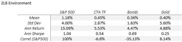
- Counter-intuitive to economic theory, when the economy requires loose monetary policy for stimulus due to underperformance, the S&P 500 is the best performing asset while when the economy does not require loose monetary policy, the S&P 500 becomes the worst-performing asset.
Introduction: Investors and PMs have traditionally used sovereign bonds as a portfolio construction and management tool for the following reasons:
- It provides a real rate of return
- Shows a high negative correlation to equity markets providing equity correction protection and portfolio diversification which improves the risk-adjusted return relationship
- High capacity, highly liquid, well-known, and understood market
Pre-ZLB Equity & Fixed-Income relationship [up to 2008-11-30] Investments 101 teaches us that equities and sovereign bonds have a high negatively correlated relationship given the risk-on, risk-off relationship between the two assets. Risk-on environments caused investors to pull money out of the safe, fixed-income assets and invest that cash in the riskier equity markets. In a risk-off environment, investors would pull their money out of the riskier equity markets and invest into the safer fixed-income market. The average FFR from 1954-07-31 to 2008-09-30 was 5.76%. This positive real yield level combined with the investor risk-on, risk-off relationship leading to equity correction protection was widely used and was a PMs most valuable portfolio construction and risk management tool. This led to the 60-40 equity-bond portfolio model template. Central Bank driven ZLB Environment Changes [2008-12-01 – Present] The ZLB environment and QE programs have significantly changed both the real yield level and the traditional relationship between equity and fixed-income markets. Since the initial move into ZLB territory towards the end of 2008, the average FFR is 0.54%. This means that PMs are returning around 90% less in terms of yield level and, when taking inflation into account, returning a negative real yield. Importantly, the medium-long term outlook for holding bonds at these yield levels is also bleak as with interest rates near 0%, there is only one way to go for interest rates and a move up will negatively effect the value of the bond holdings purchased at these levels. The market mechanics have also changed within the ZLB environment due to central bank (CB) programs. CB’s have significantly affected the capital markets over the last decade plus as they have increased money supply by levels never seen before and provided that money supply at near 0% rates. The hope was that companies invest the cheap cash in capex projects to kickstart the economy to come out of the economic recession(s). What ended up happening however was that a liquidity trap was created; with the outlook from the GFC so uncertain, companies and investors put their new, cheap money to work investing in the markets and company buybacks. Instead of investors and market participants having to pull money from their bond holdings to invest in equities, they received a new, large cash injection which they were able to invest in the equity markets without having to touch their bond holdings. At the same time this was happening, the CB became a new market participant through their QE program. While the traditional market participants invested in the equity markets, at the same time, the CB was a large buyer in the bond markets. This has changed the traditional risk-on, risk-off relationship that the traditional market participants (and Investment 101 textbooks) were used to. Given this change, PMs and investors investing their traditional 40% holding in bonds are looking at non-performing assets with a negative medium-long term outlook [rising rates] and have lost the traditional market participant risk-on, risk-off relationship. This is a dilemma that is well-known within the investment arena with very few recommendations or possible solutions on how to position a portfolio from the traditional 60-40 equity-bond template. Trend-following I analyse the CTA trend-following strategy as a potential alternative to the traditional bond holdings in a portfolio and test its return characteristics as a safe-haven type investment. In terms of high-level characteristics, I believe it is a potential solution as the strategy itself is well-known, transacts in high-capacity markets, is extremely liquid [managers provide daily liquidity] and generally has low fees for an actively managed strategy. There are two ways to be considered a safe-haven: (i) be long-only in a negatively correlated asset [like bonds or volatility] or (ii) be short equities when equities are dropping as equity portfolio holdings are generally long-only. Trend-following is dynamic as it goes both long and short markets. It also transacts across multiple, highly liquid markets including equities, fixed-income, commodities, and FX bringing with it a high degree of diversification and a high level of strategy capacity. When I put together a bucket of trend-following managers from an allocator perspective, I concentrate on 3 areas which I find are the primary drivers in the dispersion of trend-following manager’s returns: Bet Sizing There is a fantastic comparison in the capital markets and poker. Every poker player deals with the uncertainty of what the next card is going to be, just like every market participant deals with the uncertainty of the direction of the market for the next day. Over the long run, every poker player deals with the same level of uncertainty or luck in terms of what the future card(s) will be so how come there is a group of poker players who keep rising to the top? One of their biggest distinctions is their bet sizing based on the value proposition. The same can be said for trend-following managers. There is a degree of overlap between bet sizing [how much they put on for each trade given the value of the position] and the manager’s risk management framework [how much they are allowed to risk on any given position, market or time period]. Whether trend-following managers use a version of the Kelly Criterion or other bet sizing optimization models will lead to a dispersion in returns and I look to build a portfolio of diversified bet sizing optimization methods and risk-management models. Time Frame Dispersion of returns can also be seen in relation to the timeframe used to analyse trends. You cannot rationally expect a long timeframe trend-follower to capture short-term moves. Generally, the longer the timeframe of the trend analysis, the greater the beta capture within the market traded. Given the speed of equity market drops and the requirement for trend-followers to capture the drops in order to be considered a safe-haven, I focus my trend-following bucket construction on short to medium timeframe trend-following managers. Execution The speed to market and market price impact of positions is extremely important within trading as slow execution and slippage directly eats away hard-earned alpha. Given the number of markets traded and position changes within trend-following, slow trade execution can be significant to the manager’s bottom-line return percentage – as much as a couple hundred basis points. Having low slippage and execution costs will add to a manager’s bottom line performance and is something I look for. Data: Assets & Strategy This research study uses monthly data for three different assets and one alternative strategy: S&P 500 | US Bonds | Gold | CTA trend-following For the CTA trend-following proxy, I use the Nilsson Hedge CTA database. I created a trend-following index using all available trend-following manager’s monthly performances within the database. There are around 430 trend-following managers each month going back to 1983-01-01. I use an evenly weighted return for all managers that provided a return for each month to create the index. As with all indices, there will be some inherent biases with this dataset, primarily survivorship bias. For the S&P 500 proxy, I use monthly returns for the S&P 500 [Ticker=’^GSPC’]. I downloaded the data through the python API from Yahoo Finance. This data goes back to 1927-12-30. For the US bond proxy, I use the iShares 7-10-year US Bond ETF returns [Ticker=’IEF’]. I use the python API through Yahoo Finance. This data goes back to 2002-08-01. As this is an analysis for a safe-haven, I also analyse the widely considered safe-haven asset – gold. For the gold proxy, I use gold’s front-month futures price [Ticker=’CHRIS/CME_GC1’]. I use the python API through Quandl to download the gold proxy. The data goes back to 1974-12-31. As the shortest period of the data is the IEF which goes back to 2002-03-30, this research piece studies the relationship and characteristics from 2002-08-01 to present. Gold, bonds, and the S&P 500 have daily data however the trend-following index has a monthly frequency. For this reason, this research uses monthly data for all assets and strategies. Portfolio Conditions ZLB Portfolio In line with the Hughes & Rogers’ paper ‘Zero Lower Bound Monetary Policy’s Effect on Financial Asset Correlations’, we define the ZLB environment to be the months where the FFR is equal to or below 0.50%. Non-ZLB Portfolio In line with the Hughes & Rogers’ paper ‘Zero Lower Bound Monetary Policy’s Effect on Financial Asset Correlations’, we define the non-ZLB environment to be the months where the FFR is above 0.50%. As this is a study on portfolio protection during different market conditions, we also create two more portfolios:
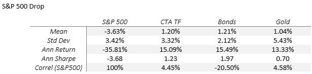
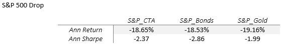
- Using month’s when the S&P 500 returns are below 0%
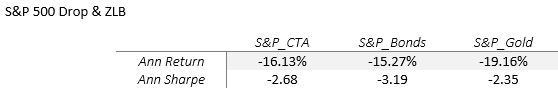
- Using months when both the S&P 500 returns are below 0% and we are within the ZLB environment.
Methodology: Equations for calculation Annualised Return = ((1 + the mean of the monthly returns during the analysis period ^ 12) – 1)) Annualised Sharpe = (the mean of the monthly returns during the analysis period / the standard deviation of the monthly returns during the analysis period) * square root (12) Correlation = Pearson Correlation Portfolio Creation The portfolio analysis section uses the traditional, widely used 60-40 portfolio construction model. The three portfolios created are: S&P 500 (60%) + CTA trend-following (40%) S&P 500 (60%) + Bonds (40%) S&P 500 (60%) + Gold (40%) Results: Individual Asset Results 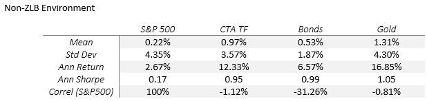
 Portfolio Results
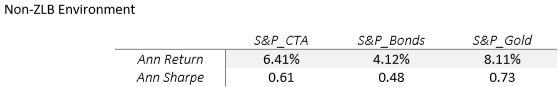
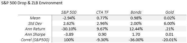
 Conclusion: Does CTA trend-following have safe-haven characteristics? US bonds and gold have long been considered capital market safe-haven assets. This is due to that traditional risk-on, risk-off relationship providing that flight to safety characteristic for bonds while gold is a precious metal used as a store of value with little economic/industrial use leading to no intrinsic value drop during economic troubles. Market participants look for a negative correlation in these assets to equities during periods of equity market drops. As the research shows, trend-following exhibits a slightly lower correlation to the S&P 500 when the S&P 500 drops than gold exhibits. In both ZLB and non-ZLB market conditions, trend-following also has a greater negative correlation to the S&P 500 than gold exhibits. Over the past two decades, trend-following has exhibited safe-haven return characteristics in line with the traditional safe-haven assets.
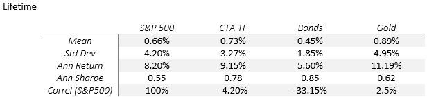
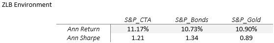
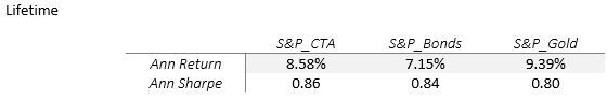
 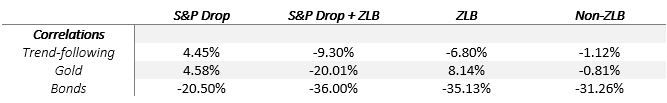 Does using trend-following as a substitute to bonds in the 60-40 model improve the portfolios performance? A good friend of mine who previously worked in Citadel Securities said to me portfolio optimization is all about reducing the risk component as it reduces the portfolio’s return expectancy. Essentially, when you add any asset with a lower return profile to a portfolio, you reduce the portfolio’s return expectancy, so you are swapping a lower return for lower level of risk. When looking at the traditional 60-40 equity-bond portfolio, this can be seen to be true through their asset’s individual lifetime returns. The S&P 500’s lifetime annualised return is 8.20% while bonds is 5.60%. If we wanted to maximise our return expectancy, we would have a 100-0 equity-bond portfolio however when we look at the best risk-adjusted performance based on the asset’s Sharpe ratio, we can see that bonds outperformed the S&P with a 0.85 versus a 0.55 Sharpe, respectively. When using a 60-40 equity-bond portfolio over the analysis lifetime instead of a 100-0 equity-bond portfolio, you get a 7.15% annualised return with a 0.84 Sharpe ratio versus an 8.20% annualised return with a 0.55 Sharpe ratio. Lower portfolio return expectancy occurs when you add an asset to a portfolio that has a lower annualised return than the current portfolio’s holdings. The traditional safe-haven of gold and my proposed new safe-haven of trend-following both have a higher return expectancy than the S&P 500 over the lifetime of this analysis at 9.15% and 11.19%, respectively versus the 8.20% for the S&P 500. Not surprisingly, the 60-40 equity-trend-following and the 60-40 equity-gold portfolio both have a lifetime portfolio return expectancy greater than the 60-40 equity-bond portfolio with 8.58% and 9.39% versus 8.20%. In terms of risk-adjusted performance of the model portfolios, the best portfolio was the equity-trend-following portfolio with an annualised Sharpe of 0.86, followed by equity-bonds with a 0.84 Sharpe followed by equity-gold with a 0.80 Sharpe. Equity – Trend-following Portfolio Outperformance The equity-trend-following portfolio, over the lifetime of the analysis period, has both a greater portfolio return expectancy and a better risk-adjusted performance versus the traditional equity-bond portfolio. An interesting counter-intuitive finding Counter intuitive to economic theory, the best performing asset when the economy requires loose monetary policy from the CB to stimulate economic growth for recovery [ZLB] is the S&P 500 while when the economy is deemed to no longer require loose monetary policy to spur growth [Non-ZLB], the S&P 500 becomes the worst performing asset.
Interested in contributing to Portfolio for the Future? Drop us a line at content@caia.org