
By Sam Holt, CFA, and Alex Billias, CFA, - Principal and Chief Operating Officer, respectively, - at the private markets consulting and advisory firm Bella Private Markets.
One of the most vexing questions in private equity is the assessment of investment returns. To extract a meaningful answer regarding its performance, a private equity group must make a number of decisions about methodology and the inclusion and exclusion of data—decisions that limited partners and consultants alike often second-guess. One might think that the process of computing an internal rate of return (IRR) or multiple of invested capital (MoIC) would be straightforward for a private equity group; it seems to be simply a matter of compiling the dates and amounts of cash flows from the firm’s investments and entering a few commands in Excel. In truth, this process is much more complex in practice.
The major challenges associated with private equity performance analysis include:
- The presence of funds at different stages of the “J-curve” in investor portfolios.
- Valuation of unrealized investments.
- The importance of using appropriate metrics and benchmarks.
The J-curve problem
The first challenge of performance benchmarking in private equity relates to which funds should and should not be included in the calculations. One might believe that an ideal return calculation should include all funds; yet there are situations in which this is not the case. We will explore why it may be preferable to exclude younger funds from this calculation.
In private equity, the term “J-curve” describes the tendency of private equity funds to report negative returns in initial years and then, in later years, post increasing returns when the investments mature.[1] In other words, the J-curve reflects a phenomenon in which a period of unfavorable returns precedes a period of gradual recovery in which the investment return (ideally) rises to a higher value than the starting point.
Figure 1 below illustrates the J-curve pattern by plotting cumulative net cash flows for vintage 2011 private equity funds. Net cash flows initially dip, reflecting the impact of fees and expenses, before increasing as the effects of the value-creation process become evident.
Figure 1: Cumulative net cash flows ($MN) vintage 2011 PE funds, by year [2]
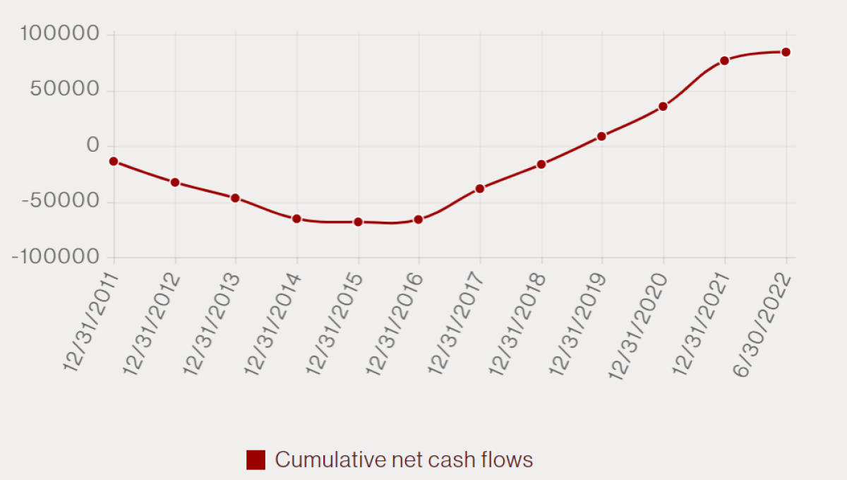
The J-curve reflects the illiquidity common to private equity. The companies that receive capital from private equity funds very often remain privately held for a number of years. As such, these companies have no observable market price. It takes many years to determine the ultimate fair price for such an investment. During this time, private equity groups will add value by, among other things, restructuring the company or making operational improvements. Funds will often hold their investments at cost for some time until these actions begin to bear fruit.
Therefore, the performance of younger funds that are early in the J-curve may not be particularly meaningful. Including young funds may thus give a misleading (negative) impression of the fund’s performance.
Groups tend to take two approaches when addressing this issue: 1) excluding funds on the basis of age (e.g., those under four years of age) or else 2) based on the share of committed capital that has been invested. The consensus in the academic literature is that both methods of exclusion are equally satisfactory (e.g., Grabenwarter and Weidig, 2005). [3]
The valuation problem
Another challenging issue with performance benchmarking involves how to assess valuations of investments that fund have not yet exited at the time of the performance assessment. In public markets, assets have clear market valuations because they are traded on liquid exchanges and real-time price information is readily available. However, this is not the case in private markets, as there is no public exchange with current prices of the privately-held assets.
Despite the illiquidity of private assets, regulations require that GPs attempt to make fair valuations. Accounting conventions such as the Financial Accounting Standards Board issued Statement 157, which encourages groups to place a value on private investments that is as close to the market price as possible. This standard requires “fair-value” reporting of assets, defined as “the price that would be received to sell an asset or paid to transfer a liability in an orderly transaction between market participants at the measurement date.”[4] Thus, “fair value” is based on the notion of an exit price (the value that would be received for a sale of the asset at the measurement date), not an entry price (the cost of the asset at the purchase date).[5] Fair value is measured by experts inside a private equity or hedge fund, or by specialized consultants. GPs (or hired experts) are relied upon to make these calculations because GPs possess the most accurate information pertaining to the assets in their portfolios.
Common valuation methods include using comparable companies, comparable transactions, and discounted cash flow analysis. While industry conventions provide guidance, valuing private companies can be difficult and subjective. Private capital often entails less frequent and inconsistent reporting compared to public markets due to lower public scrutiny and reporting requirements of the former. This leads to the “stale pricing problem,” wherein outdated valuations in private capital persist despite undocumented changes in the asset’s real value. This “smooths” out the volatility in the asset’s real price, and artificially lowers correlations between private and public markets. Therefore, it is natural for limited partners to fear that the information gaps (asymmetries) regarding portfolio company valuations create an opportunity for inaccurate valuations, which can significantly impact performance calculations.
Even with this difficulty and subjectivity, research suggests private market valuations are relatively reliable. For example, research has shown that net asset values (“NAVs”) reported by fund managers generally provide reliable indicators of the value of a fund’s investments, and fund managers have strong incentives (including reputation and the ability to raise subsequent funds) to report accurate NAVs.[6] More specifically, Brown et al. (2018) show that NAV manipulation is largely constrained to under-performing managers who are unlikely to raise follow-on funds for that very reason.[7] These findings are also corroborated by Barber and Yasuda (2017) who also find that inflated NAVs are only seen among low-reputation fund managers.[8] Taken together, these studies suggest that commonly used private market valuations are generally accurately reported by nearly all PE fund managers.
The importance of using appropriate metrics and benchmarks
An additional consideration that can make performance benchmarking problematic concerns which among many metrics and methodologies to use. Each has benefits and drawbacks, ranging from the choice of metrics to their implementation.
Metrics
The most common, “traditional” private equity performance measures include Internal Rate of Return (IRR) and cash-on-cash returns (or multiple on invested capital (MOIC)).
IRR accounts for the time value of money and can measure the performance of a series of uneven positive or negative cash flows. Investments with the highest IRRs are typically considered the most successful; however, downsides (such as the disproportionate weight IRR gives to quickly exited deals and the “reinvestment assumption”, among others)[9] can make the IRR problematic. Despite such limitations, IRR remains an industry standard for assessing prior and ongoing investments.
MOIC, however, expresses as a multiple how much a private equity fund has made on the realization of a gain on an investment, relative to how much they paid for the investment. For example, if a private equity company reports an MOIC of 1.8, the gain is 1.8 times greater than the original invested capital. In other words, it refers to the ratio of money returned and / or currently in the fund to the money invested. MOIC, however, does not take into account the time value of money, which is why this metric is usually calculated alongside others.
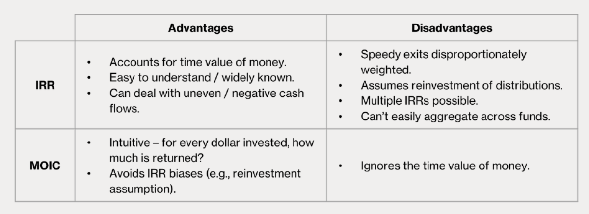
Both IRR and MOIC multiple have advantages and drawbacks, which are summarized in Table 1 below.
Table 1: Advantages and disadvantages of IRR and MOIC
Given the complexities of these metrics, and others involved in performance benchmarking, a comprehensive analysis of private equity returns requires a consideration of both measures in tandem. A “big tent approach” allows for a more holistic and thoroughly considered conclusion.
Approaches to private and public market benchmarking
A private equity firm’s calculated performance is of relatively little value until it is compared against the returns that could be received elsewhere. Two approaches are often used to undertake such comparisons. The first is to compare these returns to private equity performance benchmarks; the second is to compare them to the returns from public markets.
- Private market benchmarking
Private equity funds are typically benchmarked against other funds of the same vintage year (for example, a vintage 2003 fund will be benchmarked against other 2003 vintage funds). However, different private equity groups and data providers define vintage year in different ways: the year in which a fund is closed; the year of a fund’s first draw-down; or the year of a fund’s first investment. These are all used by different private equity groups and private equity data providers. It is therefore important to maintain a consistent definition of vintage year when calculating and benchmarking performance so that it is a “like-for-like” comparison.
There are two other immediate problems with private equity benchmarking to consider:
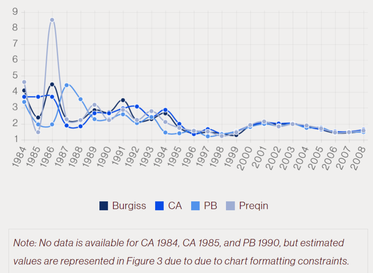
- The first is disparities among commercial private equity benchmarks. Private equity firms often provide limited information about the performance of their investments, and information gleaned from public sources about these funds is often inconsistent. As a result, benchmarks compiled by leading data service providers can differ substantially depending on the specific funds they track. Which of these benchmark data providers accurately reflect the private equity industry as a whole is a controversial issue among researchers and practitioners alike (see the discussion in Harris et al. 2014).[10] However, Brown et al. (2015)[11] examined private equity performance around the globe using four data sets from four leading commercial sources (Burgiss, Cambridge Associates (CA), PitchBook (PB) and Preqin) and found similarity in performance across the data sets (see Figure 2 and Figure 3 below), particularly in more recent years, suggesting that these issues may be lessening as data reporting improves.
Figure 2: Weighted average investment multiples for North American Venture funds, 1984-2010
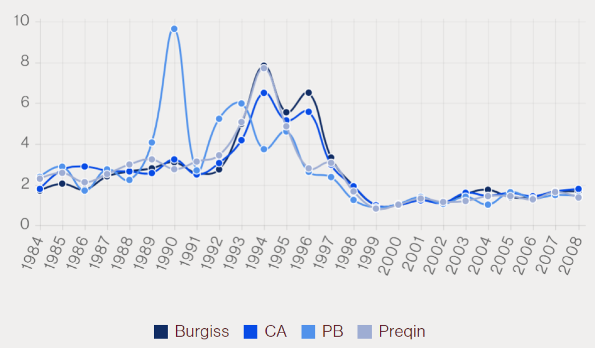
Figure 3: Weighted average investment multiples for North American Buyout funds, 1984-2010
The second problem is the failure of comparisons against benchmarks to adjust for the investments’ risk. By comparing the differences between the performance of the investments and the benchmarks, one implicitly assumes that the leverage and other risk measures for the transactions are comparable to those of the benchmarks. Thus, it is important to match the benchmarks by type of investment and geography where possible.
When comparing performance at the portfolio-level, the situation can become even more complex: there are multiple funds raised in different vintage years, potentially spanning different strategies and geographies. To compute a suitable benchmark, information from multiple years and fund types must be aggregated.
A simple approach for addressing this issue is to take a weighted average of the benchmark index. Consider the simple case of benchmarking a portfolio containing funds of the same strategy and geographic focus spanning multiple vintage years. In this case, a weighted average benchmark would be constructed wherein the weights correspond to the amount that the group invested in each given vintage (see, for instance, Fang et al. 2015).[12] Thus, had a group invested $1 billion in two funds, vintages 2002 and 2005 respectively; and $2 billion in a vintage 2007 fund, the composite return would be an average consisting of 25% each of the 2002 and 2005 benchmarks, and 50% of the 2007 benchmark.
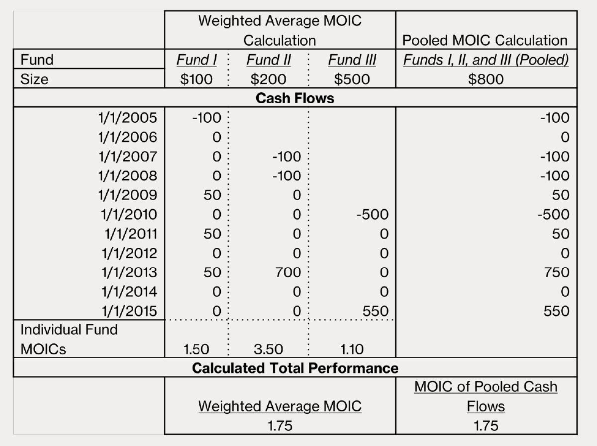
A simple weighted average, as described above, is the proper approach when benchmarking MOICs because they behave well when aggregated. As illustrated in Figure 4, the weighted average of a collection of MOICs is equal to the MOIC of the pooled cash flows, where “pooled” refers to combining all cash flows together into one hypothetical fund structure or vehicle.
Figure 4: Weighted versus pooled MOICs
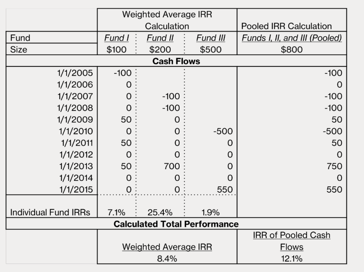
This same method, however, is not applicable when evaluating IRRs. Unlike MOICs, the weighted average of a set of IRRs is not equal to the IRR of the pooled cash flows. This issue is illustrated in Figure 5.
Figure 5: Weighted versus pooled IRRs
The preferable methodology is to calculate the pooled IRR of all the group’s funds, and then compare it to the IRR of the pooled, weighted cash flows for each benchmark. Undertaking such a calculation is difficult because few data providers grant access to the detailed benchmark cash flows or allow users to assign custom weights to the cash flows of different vintages when calculating benchmark IRRs.
2. Public market benchmarking
Certainly, such a comparison is important when assessing relative performance within a given asset class, but many entities want to compare the results of private equity investments to other asset classes. In particular, it is natural to wonder how the performance of private equity compares to that of public equity, since many institutions will reduce their public equity allocation when making private equity commitments.
Initially, one might think one could undertake this assessment by comparing the returns of private equity investments to those of a public market index over the same time period. For instance, one might compare private equity returns over a decade-and-a-half period to that of the MSCI Global Index or the S&P 500 over the same period.
But this comparison is at least somewhat—and perhaps even substantially—deceptive. Private equity has seen a torrent of funding over the past decade, making far more capital available to private equity investors than was the case 15 years ago. To compare private equity performance to the aggregate public returns over a 15-year period, which essentially gives each year of public market performance equal weight, might be misleading.
These problems have led to the development of the Public Market Equivalent (PME) methodology to compare the performance of an investment in a private equity fund with that of an investment made into a public market index. First developed by Austin Long and Craig Nickels, this methodology compares the proceeds generated by investing in the private equity fund with those generated by investing the same amount in a chosen public market index.[13] If the proceeds from the private equity investments exceed the reference return from the public investment, private equity was the superior investment; if not, one reaches the opposite conclusion. In recent years, PME has become a common industry tool for assessing performance by major limited partners (see the discussions, for instance, in practitioner-authored handbooks such as Cornelius, 2011, and Kochis et al. 2009).[14]
When a fund or group of funds has a complex series of inflows and outflows, the calculations become more challenging. In practice, a substantial array of approaches to the PME has arisen in the past 15 years. To compute the returns that an equivalently timed strategy of investing in public market securities would have produced, there are three primary methodologies: the Long-Nickels approach, Kaplan-Schoar approach, and Direct Alpha approach.
The Long-Nickels approach is the earliest PME methodology (the details of the calculations in these instances are explained in Long and Nickels (1996)[15]). Its PME calculations are undertaken by first identifying the set of cash flows from a private equity fund one wishes to assess, and the public market benchmark one wishes to use. Essentially, the calculation entails purchasing shares of the index equivalent to the amount drawn down from the private equity fund, and then selling the index at the time of each distribution. The purchase and sales are equal to the size of the private equity cash flows: thus, if the index has gone up, fewer shares are purchased. But this method, as logically appealing as it appears, has some important limitations. In particular, if private equity significantly outperforms the public markets (which literature such as Harris et al. (2019)[16] suggests is often the case), the public market portfolio will eventually become negative: one will have sold more shares than one started with. Essentially, the comparison will then become one of private equity returns with a portfolio of shorted public stocks, a comparison that does not make sense. In this case, a private equity fund that performed reasonably well during a period of sharp public market decline would be less appealing than one with the same performance during a period of public market gains. As a result, it only works in a limited set of circumstances.
The Kaplan-Schoar PME uses the returns of the public market index to discount the value of the private equity fund’s cash flows. The discounted cash outflows plus the discounted final residual value are then divided by the discounted cash inflows. This produces a ratio that indicates whether the fund outperformed or underperformed the chosen public market index. A value greater than 1.0 means the private equity fund outperformed the index and vice versa. Sorensen and Jagannathan (2013)[17] presents the theoretical rationale for this measure. It does not incur the same issues as Long-Nickels. Nonetheless, the measure is more challenging to interpret: the calculation looks at the ratio between the discounted outflows vs. inflows. While the ratio can be interpreted as the relative outperformance of private to public investments, it is less intuitive than an annual rate of return.
Complementary to the Kaplan-Schoar approach is the generalized public market equivalent G(PME) approach of Korteweg and Nagel (2016), which has better statistical properties than the ratio of discounted distributions to contributions used in prior research.[18] In effect, the G(PME) relaxes some of the assumptions of PME, such as no adjustment for risk aversion. A distinct benefit of this approach is that a G(PME) of a portfolio of funds will be the same as the weighted average of the individual funds G(PME)s – an feature not necessarily true elsewhere. While GPME works well when averaged across many funds, the performance metric is noisy for individual funds. Therefore, although this measure works well for large data sets that include funds of many varying vintages, the Kaplan-Schoar approach is typically preferable in practice.
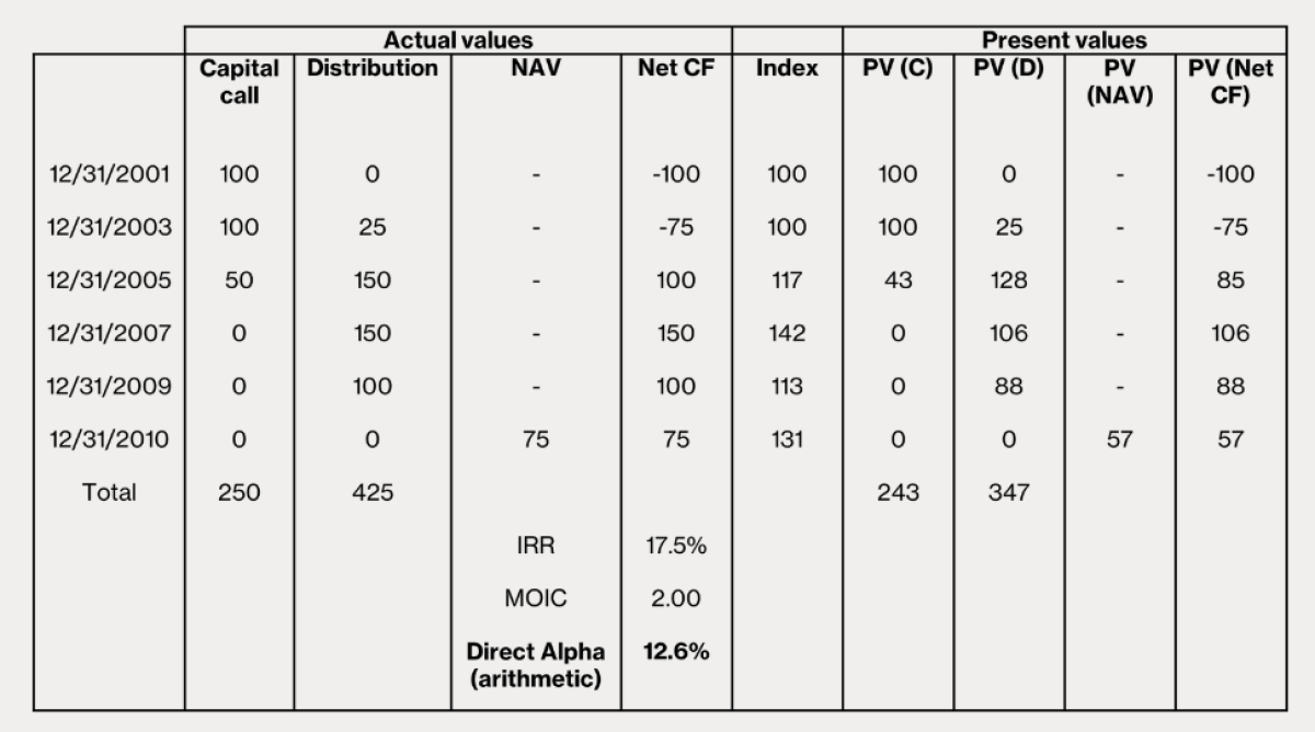
The Direct Alpha PME measures the private equity fund’s outperformance versus a public market index (see Gredil, et al (2016)[19]; Griffiths and Stucke (2014)[20]). Knowing what we know today about a certain index’s return, it calculates the money-weighted gain or loss from investing in the fund relative to the index. More specifically, the methodology involves discounting inflows and outflows from a private equity fund, using the returns of the relevant public market index as a discount rate. The methodology then computes the IRRs of the discounted net cash flows. The calculation thus piggybacks on the Kaplan-Schoar methodology but seeks to transform the outperformance (or underperformance) of the fund into a rate of return (see Table 2).
Table 2: Direct Alpha calculation
Put another way, one can think of the Direct Alpha as annualizing the Kaplan-Schoar PME and being zero whenever the Kaplan-Schoar PME is one.[21]
Conclusions
The assessment of private equity performance is a challenging exercise, due to the inherent complexities of valuation and cash flow timing. Despite its challenges, however, measuring returns in private equity remains top-of-mind, particularly as the asset class matures and sophisticated investors demand more detailed explanations of performance. The regulatory landscape has also begun to reflect its importance. For instance, in August of 2022, the SEC issued a mandate requiring the accurate and nuanced presentation of performance data in marketing materials (U.S. Securities and Exchange Commission, 2022).[22]
Given this regulatory pressure and scrutiny from sophisticated investors, private market benchmarking has rarely been more pressing. Dr. Josh Lerner and his firm, Bella Private Markets, can meet this need with experience and rigor. Please contact us at info@bella-pm.com for more information or help with private market benchmarking.
[1] Meyer, T., and P. Mathonet, 2005, Beyond the J Curve: Managing a Portfolio of Venture Capital and Private Equity Funds, New York, John Wiley & Sons.
[2] Cambridge Associates data obtained via Refinitiv on November 9, 2022; Global PE includes funds of Venture, Buyout and Growth strategies across all regions covered by Cambridge Associates.
[3] U. Grabenwarter, and T. Weidig, 2005, Exposed to the J Curve: Understanding and Managing Private Equity Fund Investments, London, Euromoney Books.
[4] Statement of Financial Accounting Standards No. 157, Paragraph 5, Financial Accounting Standards Board.
[5] Statement of Financial Accounting Standards No. 157, as elaborated in “Fair value measurement”, EY, Revised July 2018.
[6] Gregory Brown, Oleg Gredil, and Steven Kaplan; “Do Private Equity Funds Manipulate Reported Returns?”, National Bureau of Economic Research, published in Journal of Financial Economics, 2019; Brad Barber and Ayako Yasuda; “Interim Fund Performance and Fundraising in Private Equity,” Journal of Financial Economics, 2017, vol. 124, issue 1, 172-194; Tim Jenkinson (University of Oxford, Saïd Business School), Miguel Sousa (University of Porto), and Rüdiger Stucke (University of Oxford, Saïd Business School), “How Fair are the Valuations of Private Equity Funds?” February 2013, available at SSRN: https://ssrn.com/abstract=2229547
[7] Gregory Brown, Oleg Gredil, and Steven Kaplan, “Do Private Equity Funds Manipulate Reported Returns?” Journal of Financial Economics, (2018).
[8] Brad Barber and Ayako Yasuda, “Interim Fund Performance and Fundraising in Private Equity,” Journal of Financial Economics, (2017).
[9] IRR assumes reinvestment of interim cash flows in projects with equal rates of return. Therefore, IRR overstates the annual equivalent rate of return for a project that has interim cash flows which are reinvested at a lower rate than the calculated IRR. This presents a problem since there is frequently not another project available in the interim that can earn the same rate of return as the first project and can lead to major capital budget distortions.
[10] Aside from the consensus that the Thomson VentureXpert benchmark appears to be depressed in certain years (see Stucke, 2012), the question of which benchmark is best remains a matter of dispute.
[11] George W. Brown, Robert S. Harris, Tim Jenkinson, Steven N. Kaplan, and David T. Robinson, “What Do Different Commercial Data Sets Tell Us about Private Equity Performance?” SSRN, December 14, 2015, https://papers.ssrn.com/sol3/papers.cfm?abstract_id=2701317.
[12] L. Fang, V. Ivashina, and J. Lerner, 2015, “The Disintermediation of Financial Markets: Direct Investing in Private Equity,” Journal of Financial Economics, 116, 160–178, http://www.sciencedirect.com/science/article/pii/S0304405X14002724.
[13] Long, A., and C. Nickels, 1996, “A Method for Comparing Private Market Internal Rates of Return to Public Market Index Returns,” Alignment Capital (http://www.alignmentcapital.com/pdfs/research/icm_aimr_benchmark_1996.p…).
[14] Cornelius, P., 2011, International Investments in Private Equity, New York, Academic Press; Kochis, J., J. Bachman, A. Long, and C. Nickels, 2009, Inside Private Equity, New York, John Wiley & Sons.
[15] Long, A., and C. Nickels, 1996, “A Method for Comparing Private Market Internal Rates of Return to Public Market Index Returns,” Alignment Capital (http://www.alignmentcapital.com/pdfs/research/icm_aimr_benchmark_1996.p…).
[16] R. Harris, T. Jenkinson, and S. Kaplan, “Has persistence persisted in private equity? Evidence from buyout and venture capital funds,” National Bureau of Economic Research.
[17] Sorensen, M. and R. Jagannathan, 2013, “The Public Market Equivalent and Private Equity Performance,” Netspar Discussion Papers, (https://www8.gsb.columbia.edu/financialstudies/sites/financialstudies/f…).
[18] Korteweg, Arthur G. and Nagel, Stefan, “Risk-Adjusted Returns of Private Equity Funds: A New Approach,” July 8, 2022, available at SSRN: https://ssrn.com/abstract=4157952.
[19] G. Brown, Gredil O., and Kaplan S, 2016, “Do Private Equity Funds Manipulate Reported Returns?” National Bureau of Economic Research, https://www.sciencedirect.com/science/article/abs/pii/S0304405X18303015….
[20] B. Griffiths, R. Stucke, and I. Charles, “An ABC of PME,” Landmark Partners Private Equity Brief, March 2014, https://www.secondariesinvestor.com/wp-content/uploads/sites/3/2014/03/….
[21] There are a variety of alternative methodologies we do not employ. One of these is the PME+ approach (Rouvinez, 2003, 2003-04). Essentially, to avoid the shorting problem, the PME+ calculation adjusts the distributions by a factor lambda, which ensures that the ending balance of the public market portfolio does not exceed the final value of the private equity NAV. As long as the distributions from the private equity fund are not too large, the adjustment factor will be 1: in other words, all sales of the public equities will equal the outflows from the private equity fund. But if the private equity fund has very substantial distributions, the lambda factor will scale down: for instance, each distribution may only be 70% of the expected size. Rouvinez, C., 2003, “Private Equity Benchmarking with PME+,” Venture Capital Journal, (August), 34-38 (http://www.capital-dynamics.com/newswriter_files/private-equity-interna…); Rouvinez, C., 2003-04, “Beating the Public Market,” Private Equity International, __ (December/January), 26-28 (http://www.capdyn.com/newswriter_files/private-equity-international-dec…).
[22] U.S. Securities and Exchange Commission. “SEC Adopts Pay versus Performance Disclosure Rules,” August 25, 2022. https://www.sec.gov/news/press-release/2022-149.
About the Authors:
Sam Holt, CFA, a principal at Bella Private Markets, first started at Bella in 2017 and contributed to a wide variety of projects until 2020, when he left Bella as an associate. From 2020 to 2022, Sam worked as an economic and financial data analyst at the Committee of Capital Markets Regulation before returning to Bella as a principal in July 2022.
Sam has developed a keen interest in performance analysis, impact measurement, and generally how to combine qualitative and quantitative methods to derive insights for clients.
Sam graduated with an undergraduate degree from the University of Kentucky with a double major in history and philosophy. After graduating, he spent a year in a small Costa Rican community teaching English and working on various community development projects. He later received a master’s from Johns Hopkins School of Advanced International Studies focused on international relations and economics. Congruent with his studies, Sam interned in the Global Economics Group of the United States Treasury.

Alex Billias, CFA, is Chief Operating Officer at the private markets consulting and advisory firm Bella Private Markets. He also leads Bella’s efforts in developing quantitative tools, including portfolio cash flow simulation and performance benchmarking software.
At Bella, Alex has worked on projects ranging from research into the representation and performance diverse-owned firms to strategic consulting initiatives for leading global private equity and venture capital firms seeking to position themselves for success.
He completed a master’s program from Boston University’s Questrom School of Business, where he worked on management consulting projects for companies including Fidelity and ThermoFisher Scientific. Prior to graduate school, Alex obtained his bachelor’s from Boston University in Philosophy and Physics. Alex’s undergraduate research included performing Mossbauer Spectroscopy for the ISOLDE Collaboration at CERN in Geneva, publishing work investigating novel uses for organic waste materials, and composing his senior thesis “Superdeterminism and Free Will in Quantum Mechanics.”